4 Chapter 14

This is the code for Chapter 14

4.1 Program 14.1

ranks <- nhefs %>% 
  mutate(
    rank = min_rank(desc(wt82_71)), 
    lbl = if_else(
      rank <= 3 | rank >= (max(rank, na.rm = TRUE) - 2),
      round(wt82_71, 1),
      NA_real_
    )
  ) %>% 
  select(seqn, rank, lbl, wt82_71)

ranks %>% 
  select(-lbl) %>% 
  top_n(5, wt82_71)

## # A tibble: 5 x 3
##    seqn  rank wt82_71
##   <dbl> <int>   <dbl>
## 1  1769     3    37.7
## 2  5415     5    34.0
## 3  6928     2    47.5
## 4 22342     4    37.0
## 5 23522     1    48.5

ranks %>% 
  select(-lbl) %>% 
  top_n(-5, wt82_71)

## # A tibble: 5 x 3
##    seqn  rank wt82_71
##   <dbl> <int>   <dbl>
## 1  5412  1563   -29.0
## 2 13593  1565   -30.5
## 3 21897  1562   -26.0
## 4 23321  1566   -41.3
## 5 24363  1564   -30.1

ranks %>% 
  ggplot(aes(y = rank, x = wt82_71)) +
    geom_vline(xintercept = 0, col = "grey90", size = 1.3) +
    geom_point(col = "#0072B2", size = 1, alpha = .9) +
    ggrepel::geom_text_repel(
      aes(label = lbl), 
      size = 4,
      point.padding = 0.1, 
      box.padding = .6, 
      force = 1.,
      min.segment.length = 0, 
      seed = 777
    ) +
    theme_minimal(14) + 
    expand_limits(y = c(-200, 1700)) +
    xlab("change in weight")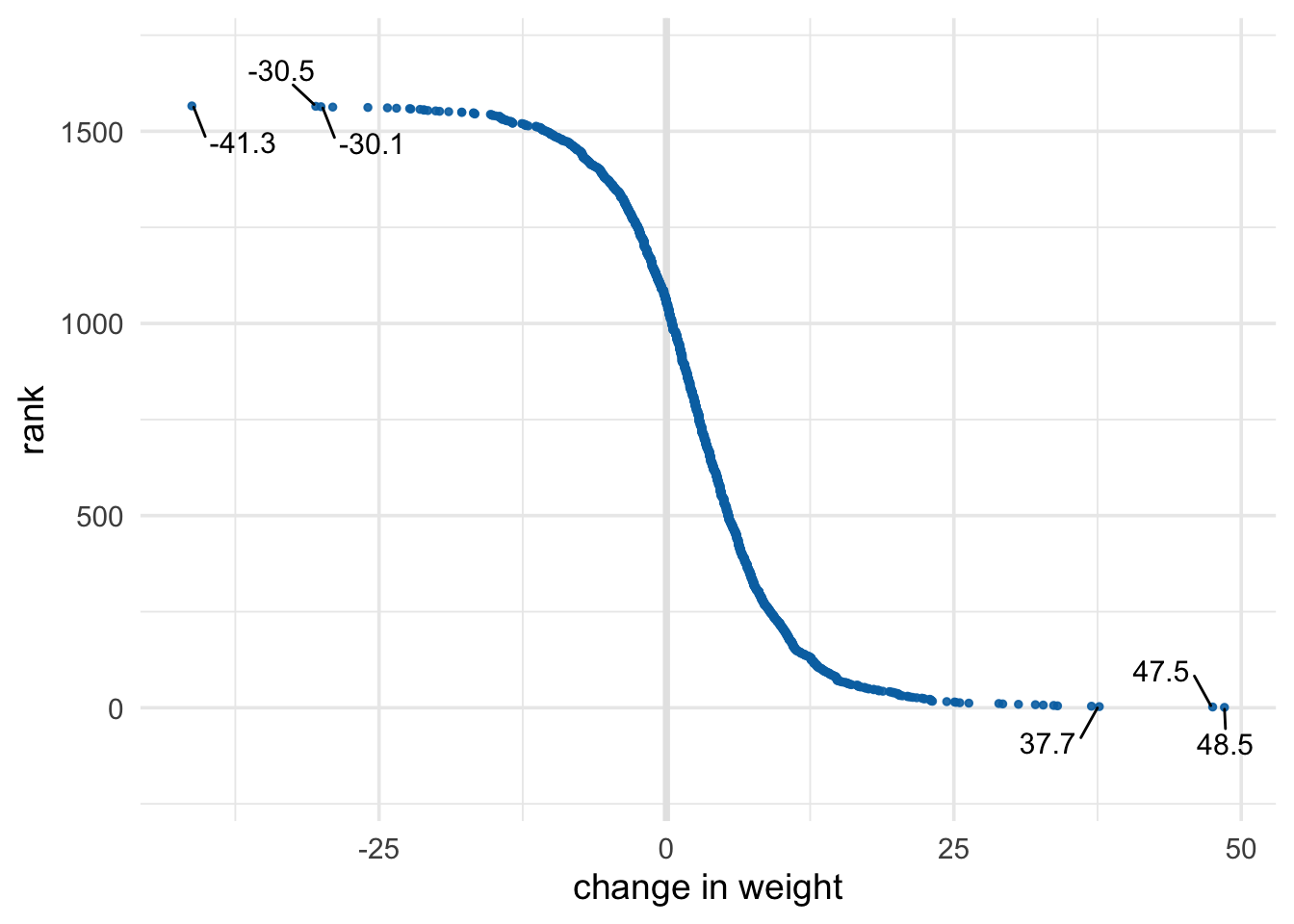

4.2 Program 14.2

# using complete data set
nhefs_censored <- nhefs %>% 
  drop_na(qsmk, sex, race, age, school, smokeintensity, smokeyrs, exercise, 
         active, wt71)

#  compute unstabilized inverse probability of censoring weights
cwts_model <- glm(
  censored ~ qsmk + sex + race + age + I(age^2) + education + 
  smokeintensity + I(smokeintensity^2) + 
  smokeyrs + I(smokeyrs^2) + exercise + active + 
  wt71 + I(wt71^2), 
  data = nhefs_censored, family = binomial()
)

nhefs_censored <- cwts_model %>% 
  augment(type.predict = "response", data = nhefs_censored) %>% 
  mutate(cwts = 1 / ifelse(censored == 0, 1 - .fitted, .fitted))

# compute all values of h(psi)
compute_h_psi <- function(psi) {
  df <- nhefs_censored %>% 
    mutate(h_psi = wt82_71 - psi * qsmk) %>% 
    # gee doesn't like missing values
    drop_na(h_psi)
  
  geeglm(
    qsmk ~ h_psi + sex + race + age + I(age^2) + education + 
      smokeintensity + I(smokeintensity^2) + 
      smokeyrs + I(smokeyrs^2) + exercise + active + 
      wt71 + I(wt71^2), 
    data = df, 
    family = binomial(),
    std.err = "san.se",
    weights = cwts, 
    id = id, 
    corstr = "independence"
  ) %>% 
    tidy() %>% 
    filter(term == "h_psi") %>% 
    mutate(psi = psi) %>% 
    select(psi, estimate, p.value)
}

compute_h_psi(3.446)

## # A tibble: 1 x 3
##     psi    estimate p.value
##   <dbl>       <dbl>   <dbl>
## 1  3.45 -0.00000190   1.000

psi_search <- map_dfr(seq(2, 5, by = .1), compute_h_psi)

psi_search %>% 
  arrange(abs(estimate))

## # A tibble: 31 x 3
##      psi  estimate p.value
##    <dbl>     <dbl>   <dbl>
##  1   3.4  0.000862   0.922
##  2   3.5 -0.00102    0.909
##  3   3.3  0.00274    0.755
##  4   3.6 -0.00290    0.744
##  5   3.2  0.00461    0.598
##  6   3.7 -0.00480    0.592
##  7   3.1  0.00647    0.457
##  8   3.8 -0.00670    0.457
##  9   3    0.00833    0.337
## 10   3.9 -0.00860    0.342
## # … with 21 more rows

psi_est <- psi_search %>% 
  arrange(abs(estimate)) %>% 
  slice(1) %>% 
  select(-estimate, -p.value)

# get minimum and maximum values that have p >= .05 for confidence intervals
psi_conf_int <- psi_search %>% 
  filter(p.value >= .05) %>% 
  slice(c(1, n())) %>% 
  mutate(type = c("conf.low", "conf.high")) %>% 
  select(type, psi) %>% 
  spread(type, psi)

bind_cols(psi_est, psi_conf_int)

## # A tibble: 1 x 3
##     psi conf.high conf.low
##   <dbl>     <dbl>    <dbl>
## 1   3.4       4.4      2.6

psi_search %>% 
  ggplot(aes(x = psi, y = estimate)) +       
    geom_hline(yintercept = 0, col = "grey85", size = 1.3) +
    geom_line(col = "#0072B2", size = 1.2) + 
    geom_point(shape = 21, col = "white", fill = "#0072B2", size = 2.5) + 
    theme_minimal(14)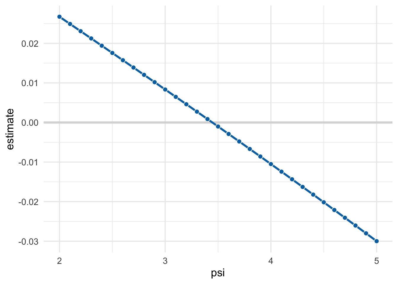

psi_formula <- function(weights, outcome, treatment, treatment_pred) {
  numerator <- weights * outcome * (treatment - treatment_pred)
  denominator <- sum(weights * treatment * (treatment - treatment_pred), na.rm = TRUE)
  sum(numerator / denominator, na.rm = TRUE)
}

estimate_psi <- function(.data) {
  glm(
    qsmk ~ sex + race + age + I(age^2) + education + 
      smokeintensity + I(smokeintensity^2) + 
      smokeyrs + I(smokeyrs^2) + exercise + active + 
      wt71 + I(wt71^2), 
    data = .data, 
    family = binomial(),
    weights = cwts, 
  ) %>% 
    augment(data = .data, type.predict = "response") %>% 
    summarize(
      psi = psi_formula(
        weights = cwts, 
        outcome = wt82_71, 
        treatment = qsmk, 
        treatment_pred = .fitted
      )
    )
}

nhefs_censored %>% 
  select(-.fitted:-.cooksd) %>% 
  filter(censored == 0) %>% 
  estimate_psi()

## # A tibble: 1 x 1
##     psi
##   <dbl>
## 1  3.45

bootstrap_psi <- function(data, indices) {
  estimate_psi(data[indices, ]) %>% pull(psi)
}

bootstrapped_psis <- nhefs_censored %>% 
  select(-.fitted:-.cooksd) %>% 
  filter(censored == 0) %>% 
  boot(bootstrap_psi, R = 2000)

bootstrapped_psis %>% 
  tidy(conf.int = TRUE, conf.method = "bca")

## # A tibble: 1 x 5
##   statistic     bias std.error conf.low conf.high
##       <dbl>    <dbl>     <dbl>    <dbl>     <dbl>
## 1      3.45 -0.00202     0.473     2.51      4.38

4.3 Program 14.3

estimate_psi2 <- function(.data) {
  glm(
    qsmk ~ sex + race + age + I(age^2) + education + 
      smokeintensity + I(smokeintensity^2) + 
      smokeyrs + I(smokeyrs^2) + exercise + active + 
      wt71 + I(wt71^2), 
    data = .data, 
    family = binomial(),
    weights = cwts, 
  ) %>% 
    augment(data = .data, type.predict = "response") %>% 
    psi_formula2()
}

solve_matrix <- function(.data, .names = c("psi1", "psi2")) {
  cells <- .data %>% 
    summarise(
      a1 = sum(qsmk * diff), 
      a2 = sum(qsmk * smokeintensity  * diff), 
      a3 = sum(qsmk * smokeintensity * diff), 
      a4 = sum(qsmk * smokeintensity * smokeintensity * diff),
      b1 = sum(wt82_71 * diff),
      b2 = sum(wt82_71 * smokeintensity * diff)
    )
  
  a <- cells %>% 
    select(a1:a4) %>% 
    unlist() %>% 
    matrix(2, 2)
  
  b <- cells %>% 
    select(b1:b2) %>% 
    unlist() %>% 
    matrix(2, 1)
  
  solve(a, b) %>% 
    t() %>% 
    as_tibble(.name_repair = "minimal") %>% 
    set_names(.names)
}

psi_formula2 <- function(.data) {
  .data %>% 
    mutate(diff = (qsmk - .fitted) * cwts) %>% 
    drop_na(wt82_71) %>% 
    solve_matrix()
}

nhefs_censored %>% 
  select(-.fitted:-.cooksd) %>% 
  filter(censored == 0) %>% 
  estimate_psi2()

## # A tibble: 1 x 2
##    psi1   psi2
##   <dbl>  <dbl>
## 1  2.86 0.0300