1 Chapter 11

This is the code for Chapter 11

1.1 Program 11.1

library(tidyverse)
library(broom)

binary_a_df <- data.frame(
  a = c(rep(1, 8), rep(0, 8)),
  y = c(200, 150, 220, 110, 50, 180, 90, 170, 
        170, 30, 70, 110, 80, 50, 10, 20)
)

ggplot(binary_a_df, aes(a, y)) +
  geom_point(size = 4, col = "white", fill = "#E69F00", shape = 21) +
  scale_x_continuous(breaks = c(0, 1), expand = expand_scale(.5)) + 
  theme_minimal(base_size = 20)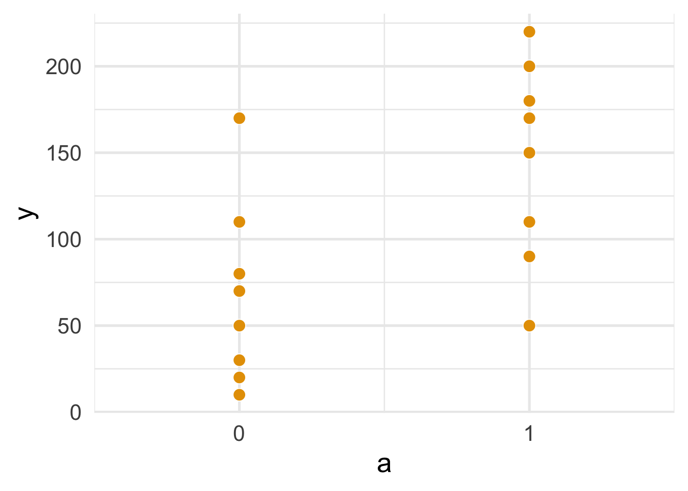

FIGURE 1.1: Figure 11.1

binary_a_df %>% 
  group_by(a) %>% 
  summarize(n = n(), mean = mean(y), sd = sd(y), 
            minimum = min(y), maximum = max(y)) %>% 
  knitr::kable(digits = 2)

a	n	mean	sd	minimum	maximum
0	8	67.50	53.12	10	170
1	8	146.25	58.29	50	220

categorical_a_df <- data.frame(a = sort(rep(1:4, 4)),
                               y = c(110, 80, 50, 40, 170, 30, 70, 50, 
                                     110, 50, 180, 130, 200, 150, 220, 210))

ggplot(categorical_a_df, aes(a, y)) +
  geom_point(size = 4, col = "white", fill = "#E69F00",  shape = 21) +
  scale_x_continuous(breaks = 1:4, expand = expand_scale(.25)) + 
  theme_minimal(base_size = 20)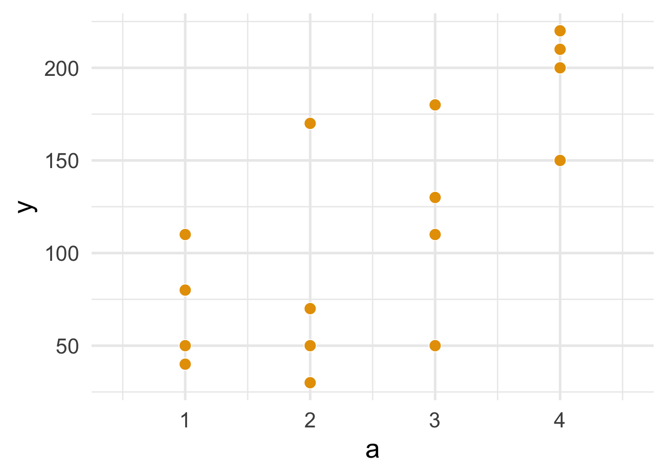

FIGURE 1.2: Figure 11.2

categorical_a_df %>% 
  group_by(a) %>% 
  summarize(n = n(), mean = mean(y), sd = sd(y), minimum = min(y), maximum = max(y)) %>% 
  knitr::kable(digits = 2)

a	n	mean	sd	minimum	maximum
1	4	70.0	31.62	40	110
2	4	80.0	62.18	30	170
3	4	117.5	53.77	50	180
4	4	195.0	31.09	150	220

1.2 Program 11.2

continuous_a_df <- data.frame(a = c(3,11,17,23,29,37,41,53,
                                    67,79,83,97,60,71,15,45),
                              y = c(21,54,33,101,85,65,157,120,
                                    111,200,140,220,230,217,11,190))


ggplot(continuous_a_df, aes(a, y)) +
  geom_point(size = 4, col = "white", fill = "#E69F00",  shape = 21) +
  theme_minimal(base_size = 20)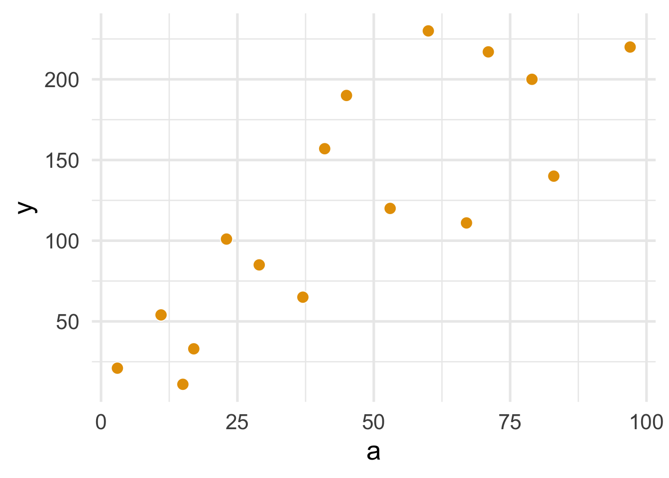

FIGURE 1.3: Figure 11.3

ggplot(continuous_a_df, aes(a, y)) +
  geom_point(size = 4, col = "white", fill = "grey85", shape = 21) +
  geom_smooth(method = "lm", se = FALSE, col = "#E69F00", size = 1.2) + 
  theme_minimal(base_size = 20)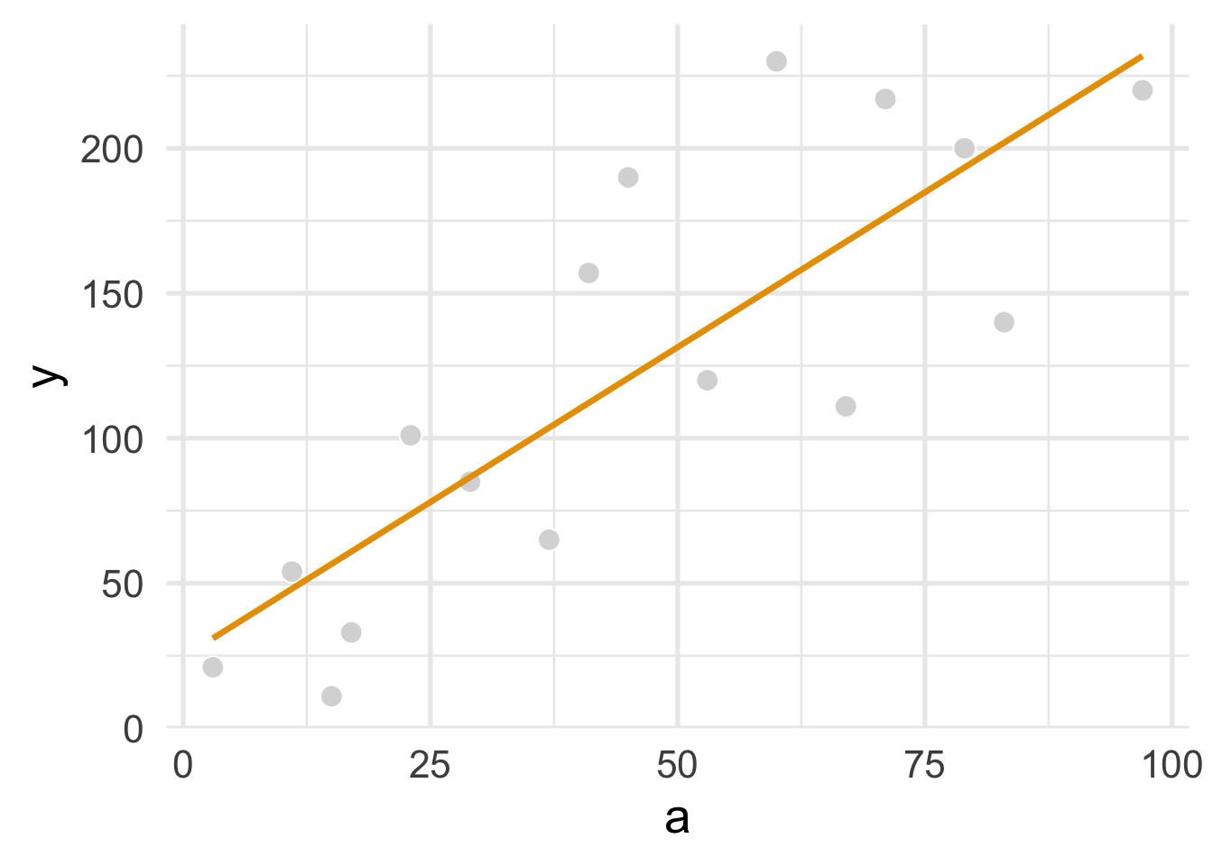 

FIGURE 1.4: Figure 11.4

linear_regression <- lm(y ~ a, data = continuous_a_df)

linear_regression %>% 
  tidy(conf.int = TRUE) %>% 
  select(-statistic, -p.value) %>% 
  knitr::kable(digits = 2)

term	estimate	std.error	conf.low	conf.high
(Intercept)	24.55	21.33	-21.20	70.29
a	2.14	0.40	1.28	2.99

linear_regression %>% 
  predict(newdata = data.frame(a = 90))

##      1 
## 216.89

lm(y ~ a, data = binary_a_df) %>% 
  tidy(conf.int = TRUE) %>% 
  select(-statistic, -p.value) %>% 
  knitr::kable(digits = 2)

term	estimate	std.error	conf.low	conf.high
(Intercept)	67.50	19.72	25.21	109.79
a	78.75	27.88	18.95	138.55

1.3 Program 11.3

smoothed_regression <- lm(y ~ a + I(a^2), data = continuous_a_df) 

smoothed_regression %>% 
  tidy(conf.int = TRUE) %>% 
  select(-statistic, -p.value) %>% 
  mutate(term = ifelse(term == "I(a^2)", "a^2", term)) %>% 
  knitr::kable(digits = 2) 

term	estimate	std.error	conf.low	conf.high
(Intercept)	-7.41	31.75	-75.99	61.18
a	4.11	1.53	0.80	7.41
a^2	-0.02	0.02	-0.05	0.01

ggplot(continuous_a_df, aes(a, y)) +
  geom_point(size = 4, col = "white", fill = "grey85", shape = 21) +
  geom_smooth(method = "lm", se = FALSE, col = "#E69F00", formula = y ~ x + I(x^2), size = 1.2) + 
  theme_minimal(base_size = 20)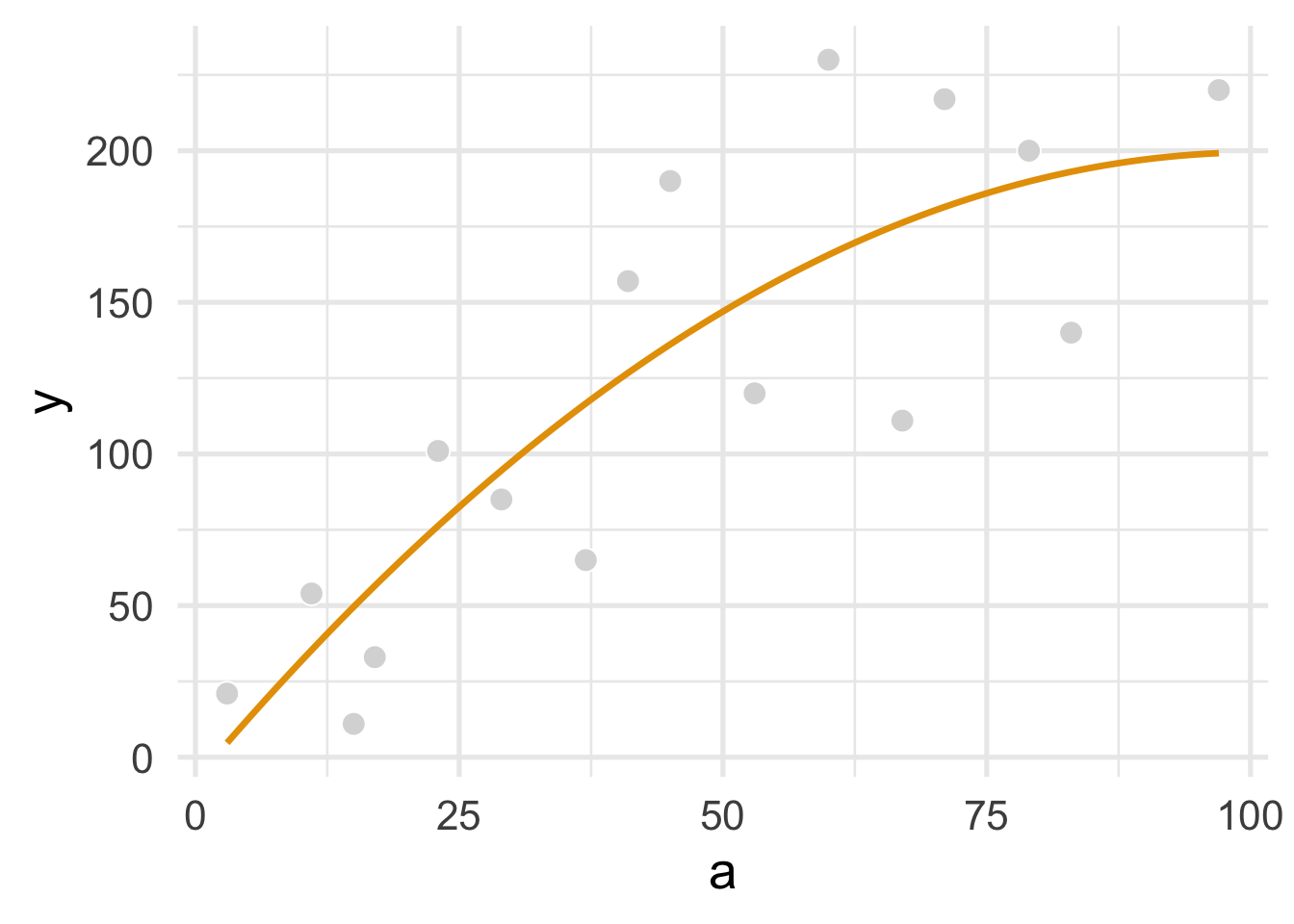 

FIGURE 1.5: Figure 11.5

smoothed_regression %>% 
  predict(newdata = data.frame(a = 90))

##        1 
## 197.1269