2 Chapter 12

This is the code for Chapter 12

2.1 Program 12.1

library(tidyverse)
library(haven)
library(broom)
library(tableone)

nhefs <- read_sas("data/nhefs.sas7bdat")

nhefs

## # A tibble: 1,629 x 64
##     seqn  qsmk death yrdth modth dadth   sbp   dbp   sex   age  race income
##    <dbl> <dbl> <dbl> <dbl> <dbl> <dbl> <dbl> <dbl> <dbl> <dbl> <dbl>  <dbl>
##  1   233     0     0    NA    NA    NA   175    96     0    42     1     19
##  2   235     0     0    NA    NA    NA   123    80     0    36     0     18
##  3   244     0     0    NA    NA    NA   115    75     1    56     1     15
##  4   245     0     1    85     2    14   148    78     0    68     1     15
##  5   252     0     0    NA    NA    NA   118    77     0    40     0     18
##  6   257     0     0    NA    NA    NA   141    83     1    43     1     11
##  7   262     0     0    NA    NA    NA   132    69     1    56     0     19
##  8   266     0     0    NA    NA    NA   100    53     1    29     0     22
##  9   419     0     1    84    10    13   163    79     0    51     0     18
## 10   420     0     1    86    10    17   184   106     0    43     0     16
## # … with 1,619 more rows, and 52 more variables: marital <dbl>,
## #   school <dbl>, education <dbl>, ht <dbl>, wt71 <dbl>, wt82 <dbl>,
## #   wt82_71 <dbl>, birthplace <dbl>, smokeintensity <dbl>,
## #   smkintensity82_71 <dbl>, smokeyrs <dbl>, asthma <dbl>, bronch <dbl>,
## #   tb <dbl>, hf <dbl>, hbp <dbl>, pepticulcer <dbl>, colitis <dbl>,
## #   hepatitis <dbl>, chroniccough <dbl>, hayfever <dbl>, diabetes <dbl>,
## #   polio <dbl>, tumor <dbl>, nervousbreak <dbl>, alcoholpy <dbl>,
## #   alcoholfreq <dbl>, alcoholtype <dbl>, alcoholhowmuch <dbl>,
## #   pica <dbl>, headache <dbl>, otherpain <dbl>, weakheart <dbl>,
## #   allergies <dbl>, nerves <dbl>, lackpep <dbl>, hbpmed <dbl>,
## #   boweltrouble <dbl>, wtloss <dbl>, infection <dbl>, active <dbl>,
## #   exercise <dbl>, birthcontrol <dbl>, pregnancies <dbl>,
## #   cholesterol <dbl>, hightax82 <dbl>, price71 <dbl>, price82 <dbl>,
## #   tax71 <dbl>, tax82 <dbl>, price71_82 <dbl>, tax71_82 <dbl>

nhefs <- nhefs %>% 
  # add id and censored indicator
  # recode age > 50 and years of school to categories
  mutate(
    id = 1:n(),
    censored = ifelse(is.na(wt82), 1, 0),
    older = case_when(is.na(age) ~ NA_real_,
                      age > 50 ~ 1,
                      TRUE ~ 0),
    education = case_when(school <  9 ~ 1,
                       school <  12 ~ 2,
                       school == 12 ~ 3,
                       school < 16 ~ 4,
                       TRUE ~ 5)
  ) %>% 
  # change categorical to factors
  mutate_at(vars(sex, race, education, exercise, active), factor)


# restrict to complete cases
nhefs_complete <- nhefs %>% 
  drop_na(qsmk, sex, race, age, school, smokeintensity, smokeyrs, exercise, 
         active, wt71, wt82, wt82_71, censored)


nhefs_complete %>%
  filter(censored == 0) %>% 
  group_by(qsmk) %>% 
  summarize(mean_weight_change = mean(wt82_71), sd = sd(wt82_71)) %>% 
  knitr::kable(digits = 2)

qsmk	mean_weight_change	sd
0	1.98	7.45
1	4.53	8.75

# clean up the data for the table
fct_yesno <- function(x) {
  factor(x, labels = c("No", "Yes"))
}

tbl1_data <- nhefs_complete %>% 
    filter(censored == 0) %>%
    mutate(university = fct_yesno(ifelse(education == 5, 1, 0)),
           no_exercise = fct_yesno(ifelse(exercise == 2, 1, 0)),
           inactive = fct_yesno(ifelse(active == 2, 1, 0)),
           qsmk = factor(qsmk, levels = 1:0, c("Ceased Smoking", "Continued Smoking")),
           sex = factor(sex, levels = 1:0, labels = c("Female", "Male")),
           race = factor(race, levels = 1:0, labels = c("Other", "White"))) %>% 
    select(qsmk, age, sex, race, university, wt71, smokeintensity, smokeyrs, no_exercise, 
           inactive) %>% 
  rename("Smoking Cessation" = "qsmk",
         "Age" = "age",
         "Sex" = "sex",
         "Race" = "race",
         "University education" = "university",
         "Weight, kg" = "wt71", 
         "Cigarettes/day" = "smokeintensity",
         "Years smoking" = "smokeyrs",
         "Little or no exercise" = "no_exercise",
         "Inactive daily life" = "inactive")

kableone <- function(x, ...) {
  capture.output(x <- print(x))
  knitr::kable(x, ...)
}

tbl1_data %>% 
  CreateTableOne(vars = select(tbl1_data, -`Smoking Cessation`) %>% names, 
                 strata = "Smoking Cessation", data = ., test = FALSE) %>% 
  kableone()

	Ceased Smoking	Continued Smoking
n	403	1163
Age (mean (sd))	46.17 (12.21)	42.79 (11.79)
Sex = Male (%)	220 (54.6)	542 (46.6)
Race = White (%)	367 (91.1)	993 (85.4)
University education = Yes (%)	62 (15.4)	115 ( 9.9)
Weight, kg (mean (sd))	72.35 (15.63)	70.30 (15.18)
Cigarettes/day (mean (sd))	18.60 (12.40)	21.19 (11.48)
Years smoking (mean (sd))	26.03 (12.74)	24.09 (11.71)
Little or no exercise = Yes (%)	164 (40.7)	441 (37.9)
Inactive daily life = Yes (%)	45 (11.2)	104 ( 8.9)

2.2 Program 12.2

# Estimation of IP weights via a logistic model

propensity <- glm(qsmk ~ sex + race + age + I(age^2) + education + 
                  smokeintensity + I(smokeintensity^2) + 
                  smokeyrs + I(smokeyrs^2) + exercise + active + 
                  wt71 + I(wt71^2), 
                  family = binomial(), data = nhefs_complete)

propensity %>% 
  tidy(conf.int = TRUE, exponentiate = TRUE) %>% 
  select(-statistic, -p.value) %>% 
  knitr::kable(digits = 2)

term	estimate	std.error	conf.low	conf.high
(Intercept)	0.11	1.38	0.01	1.56
sex1	0.59	0.15	0.44	0.80
race1	0.43	0.21	0.28	0.64
age	1.13	0.05	1.02	1.25
I(age^2)	1.00	0.00	1.00	1.00
education2	0.97	0.20	0.66	1.43
education3	1.09	0.18	0.77	1.55
education4	1.07	0.27	0.62	1.81
education5	1.61	0.23	1.03	2.51
smokeintensity	0.93	0.02	0.90	0.95
I(smokeintensity^2)	1.00	0.00	1.00	1.00
smokeyrs	0.93	0.03	0.88	0.98
I(smokeyrs^2)	1.00	0.00	1.00	1.00
exercise1	1.43	0.18	1.01	2.04
exercise2	1.49	0.19	1.03	2.15
active1	1.03	0.13	0.80	1.34
active2	1.19	0.21	0.78	1.81
wt71	0.98	0.03	0.94	1.04
I(wt71^2)	1.00	0.00	1.00	1.00

nhefs_complete <- propensity %>% 
  augment(type.predict = "response", data = nhefs_complete) %>% 
  mutate(wts = 1 / ifelse(qsmk == 0, 1 - .fitted, .fitted))
    
nhefs_complete %>% 
  summarize(mean_wt = mean(wts), sd_wts = sd(wts))

## # A tibble: 1 x 2
##   mean_wt sd_wts
##     <dbl>  <dbl>
## 1    2.00   1.47

ggplot(nhefs_complete, aes(wts)) +
  geom_density(col = "#E69F00", fill = "#E69F0095") + 
  scale_x_log10() + 
  theme_minimal(base_size = 14) + 
  xlab("log10(Weights)")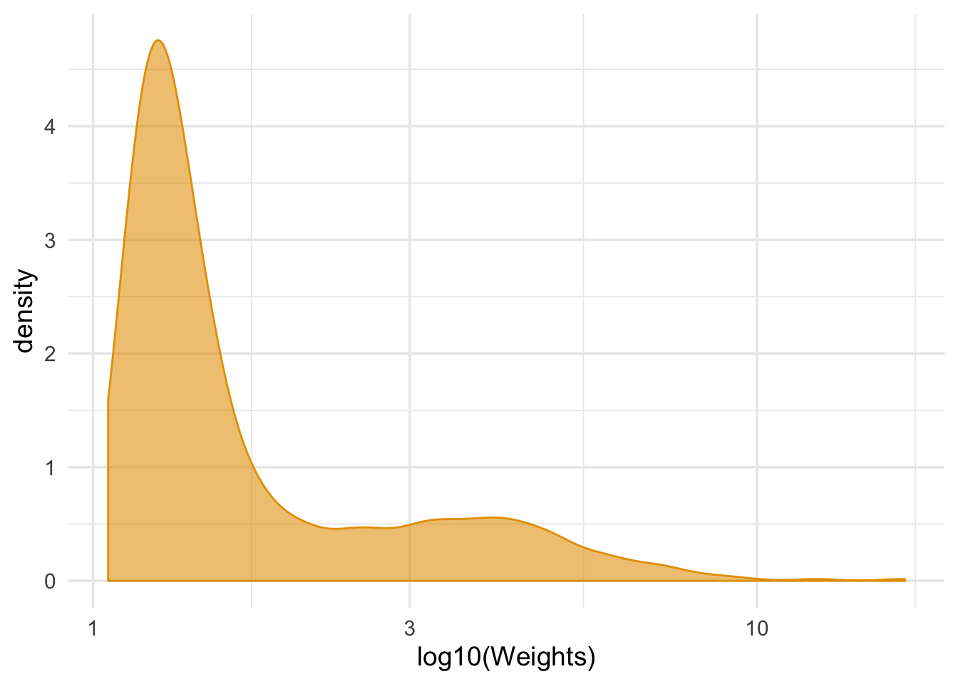

tidy_est_cis <- function(.df, .type) {
  .df %>% 
    mutate(type = .type) %>% 
    filter(term == "qsmk") %>% 
    select(type, estimate, conf.low, conf.high)
}

#  standard error a little too small
ols_cis <- lm(wt82_71 ~ qsmk, data = nhefs_complete, weights = wts) %>% 
  tidy(conf.int = TRUE) %>% 
  tidy_est_cis("ols")

ols_cis

## # A tibble: 1 x 4
##   type  estimate conf.low conf.high
##   <chr>    <dbl>    <dbl>     <dbl>
## 1 ols       3.44     2.64      4.24

library(geepack)
gee_model <- geeglm(
  wt82_71 ~ qsmk, 
  data = nhefs_complete, 
  std.err = "san.se", # default robust SE 
  weights = wts, # inverse probability weights
  id = id, 
  corstr = "independence" # independent correlation structure
) 

gee_model_cis <- tidy(gee_model, conf.int = TRUE) %>% 
  tidy_est_cis("gee")

gee_model_cis

## # A tibble: 1 x 4
##   type  estimate conf.low conf.high
##   <chr>    <dbl>    <dbl>     <dbl>
## 1 gee       3.44     2.41      4.47

#  easy robust SEs
library(estimatr)
robust_lm_model_cis <- lm_robust(
  wt82_71 ~ qsmk, data = nhefs_complete, 
  weights = wts
) %>% 
  tidy() %>% 
  tidy_est_cis("robust ols")

robust_lm_model_cis

##         type estimate conf.low conf.high
## 1 robust ols 3.440535 2.407886  4.473185

model_nhefs <- function(data, indices) {
  #  need to bootstrap the entire fitting process, including IPWs
  df <- data[indices, ]
  propensity <- glm(qsmk ~ sex + race + age + I(age^2) + education + 
                  smokeintensity + I(smokeintensity^2) + 
                  smokeyrs + I(smokeyrs^2) + exercise + active + 
                  wt71 + I(wt71^2), 
                  family = binomial(), data = df)

df <- propensity %>% 
  augment(type.predict = "response", data = df) %>% 
  mutate(wts = 1 / ifelse(qsmk == 0, 1 - .fitted, .fitted))

  lm(wt82_71 ~ qsmk, data = df, weights = wts) %>% 
    tidy() %>% 
    filter(term == "qsmk") %>% 
    pull(estimate)
}

library(boot)
set.seed(1234)

bootstrap_estimates <- nhefs_complete %>% 
  select(-.fitted:-wts) %>% 
  boot(model_nhefs, R = 2000)
bootstrap_cis <- bootstrap_estimates %>% 
  tidy(conf.int = TRUE, conf.method = "bca") %>% 
  mutate(type = "bootstrap") %>% 
  select(type, estimate = statistic, conf.low, conf.high)

bootstrap_cis

## # A tibble: 1 x 4
##   type      estimate conf.low conf.high
##   <chr>        <dbl>    <dbl>     <dbl>
## 1 bootstrap     3.44     2.47      4.43

bind_rows(ols_cis, gee_model_cis, robust_lm_model_cis, bootstrap_cis) %>% 
  mutate(width = conf.high - conf.low) %>% 
  arrange(width) %>% 
  mutate(type = fct_inorder(type)) %>% 
  ggplot(aes(x = type, y = estimate, ymin = conf.low, ymax = conf.high)) + 
    geom_pointrange(color = "#0172B1", size = 1, fatten = 3) +
    coord_flip() +
    theme_minimal(base_size = 14)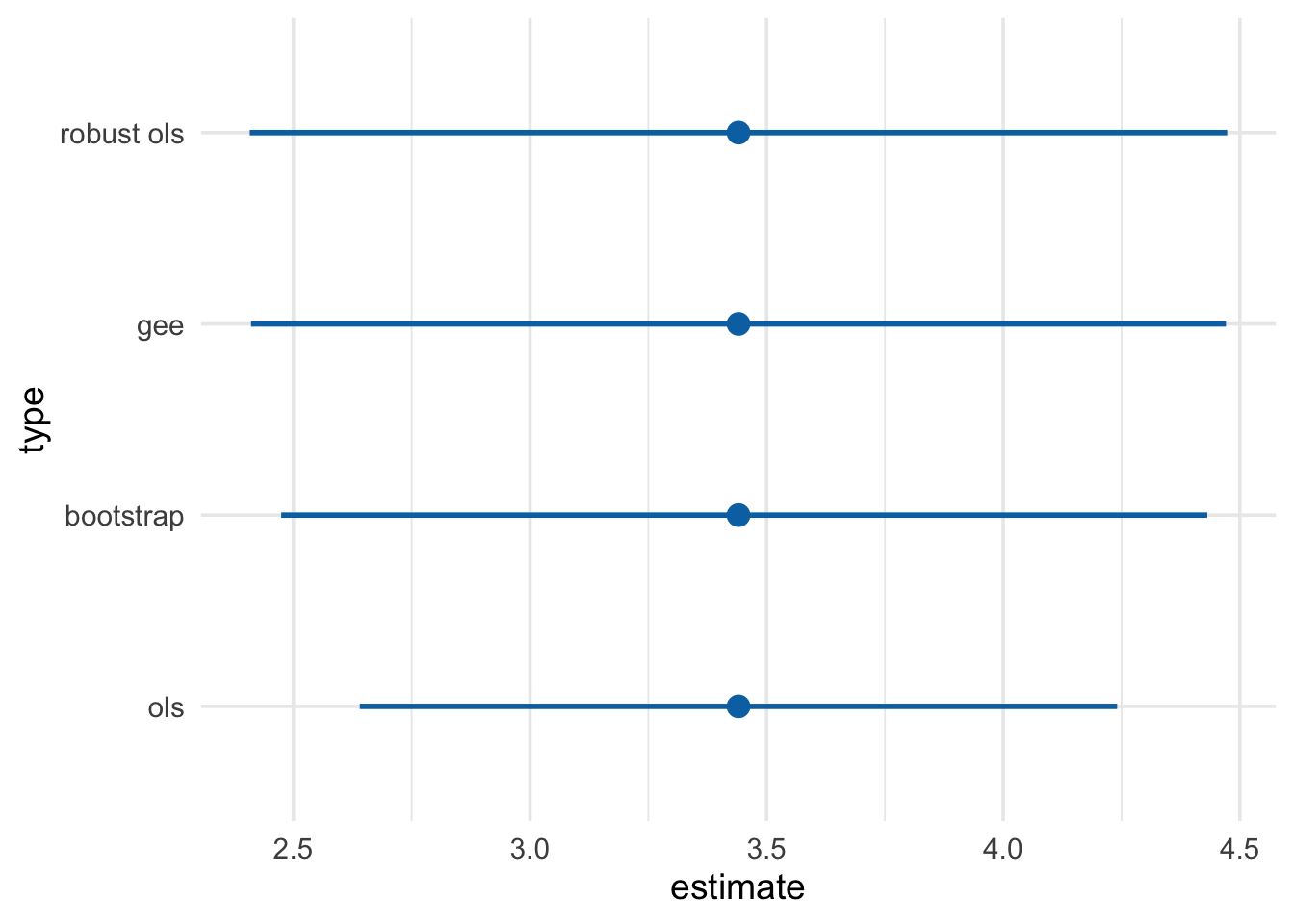

2.3 Program 12.3

numerator <- glm(qsmk ~ 1, data = nhefs_complete, family = binomial())

nhefs_complete <- numerator %>% 
  augment(type.predict = "response", data = nhefs_complete) %>% 
  mutate(numerator = ifelse(qsmk == 0, 1 - .fitted, .fitted)) %>% 
  select(id, numerator) %>% 
  left_join(nhefs_complete, by = "id") %>% 
  mutate(swts = numerator / ifelse(qsmk == 0, 1 - .fitted, .fitted))

nhefs_complete %>% 
  summarize(mean_wt = mean(swts), sd_wts = sd(swts))

## # A tibble: 1 x 2
##   mean_wt sd_wts
##     <dbl>  <dbl>
## 1   0.999  0.288

ggplot(nhefs_complete, aes(swts)) +
  geom_density(col = "#E69F00", fill = "#E69F0095") + 
  scale_x_log10() + 
  theme_minimal(base_size = 14) + 
  xlab("log10(Stabilized Weights)")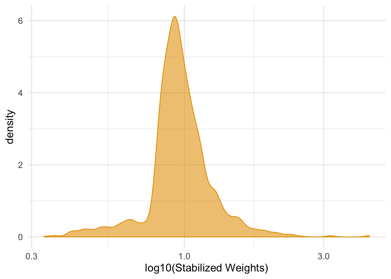

lm_robust(wt82_71 ~ qsmk, data = nhefs_complete, weights = swts) %>% 
  tidy()

##          term estimate std.error statistic      p.value conf.low conf.high
## 1 (Intercept) 1.779978 0.2248362  7.916778 4.581734e-15 1.338966  2.220990
## 2        qsmk 3.440535 0.5264638  6.535179 8.573524e-11 2.407886  4.473185
##     df outcome
## 1 1564 wt82_71
## 2 1564 wt82_71

2.4 Program 12.4

nhefs_light_smokers <- nhefs %>% 
  drop_na(qsmk, sex, race, age, school, smokeintensity, smokeyrs, exercise, 
         active, wt71, wt82, wt82_71, censored) %>% 
  filter(smokeintensity <= 25)

nhefs_light_smokers

## # A tibble: 1,162 x 67
##     seqn  qsmk death yrdth modth dadth   sbp   dbp sex     age race  income
##    <dbl> <dbl> <dbl> <dbl> <dbl> <dbl> <dbl> <dbl> <fct> <dbl> <fct>  <dbl>
##  1   235     0     0    NA    NA    NA   123    80 0        36 0         18
##  2   244     0     0    NA    NA    NA   115    75 1        56 1         15
##  3   245     0     1    85     2    14   148    78 0        68 1         15
##  4   252     0     0    NA    NA    NA   118    77 0        40 0         18
##  5   257     0     0    NA    NA    NA   141    83 1        43 1         11
##  6   262     0     0    NA    NA    NA   132    69 1        56 0         19
##  7   266     0     0    NA    NA    NA   100    53 1        29 0         22
##  8   419     0     1    84    10    13   163    79 0        51 0         18
##  9   420     0     1    86    10    17   184   106 0        43 0         16
## 10   434     0     0    NA    NA    NA   127    80 1        54 0         16
## # … with 1,152 more rows, and 55 more variables: marital <dbl>,
## #   school <dbl>, education <fct>, ht <dbl>, wt71 <dbl>, wt82 <dbl>,
## #   wt82_71 <dbl>, birthplace <dbl>, smokeintensity <dbl>,
## #   smkintensity82_71 <dbl>, smokeyrs <dbl>, asthma <dbl>, bronch <dbl>,
## #   tb <dbl>, hf <dbl>, hbp <dbl>, pepticulcer <dbl>, colitis <dbl>,
## #   hepatitis <dbl>, chroniccough <dbl>, hayfever <dbl>, diabetes <dbl>,
## #   polio <dbl>, tumor <dbl>, nervousbreak <dbl>, alcoholpy <dbl>,
## #   alcoholfreq <dbl>, alcoholtype <dbl>, alcoholhowmuch <dbl>,
## #   pica <dbl>, headache <dbl>, otherpain <dbl>, weakheart <dbl>,
## #   allergies <dbl>, nerves <dbl>, lackpep <dbl>, hbpmed <dbl>,
## #   boweltrouble <dbl>, wtloss <dbl>, infection <dbl>, active <fct>,
## #   exercise <fct>, birthcontrol <dbl>, pregnancies <dbl>,
## #   cholesterol <dbl>, hightax82 <dbl>, price71 <dbl>, price82 <dbl>,
## #   tax71 <dbl>, tax82 <dbl>, price71_82 <dbl>, tax71_82 <dbl>, id <int>,
## #   censored <dbl>, older <dbl>

denominator_model <- lm(smkintensity82_71 ~ sex + race + age + I(age^2) + education + 
                  smokeintensity + I(smokeintensity^2) + 
                  smokeyrs + I(smokeyrs^2) + exercise + active + 
                  wt71 + I(wt71^2), data = nhefs_light_smokers)

denominators <- denominator_model %>% 
  augment(data = nhefs_light_smokers) %>% 
  mutate(denominator = dnorm(smkintensity82_71, .fitted, mean(.sigma, na.rm = TRUE))) %>% 
  select(id, denominator)

numerator_model <- lm(smkintensity82_71 ~ 1, data = nhefs_light_smokers)

numerators <- numerator_model %>% 
  augment(data = nhefs_light_smokers) %>% 
  mutate(numerator = dnorm(smkintensity82_71, .fitted, mean(.sigma, na.rm = TRUE))) %>% 
  select(id, numerator)

nhefs_light_smokers <- nhefs_light_smokers %>% 
  left_join(numerators, by = "id") %>% 
  left_join(denominators, by = "id") %>% 
  mutate(swts = numerator / denominator)

ggplot(nhefs_light_smokers, aes(swts)) +
  geom_density(col = "#E69F00", fill = "#E69F0095") + 
  scale_x_log10() + 
  theme_minimal(base_size = 14) + 
  xlab("log10(Stabilized Weights)")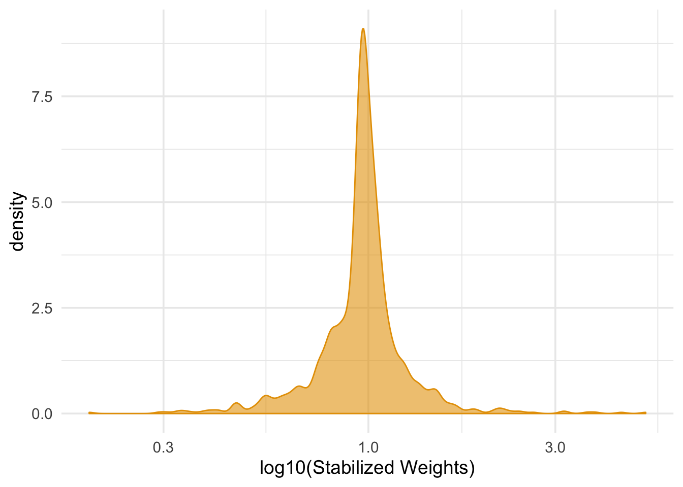

smk_intensity_model <- lm_robust(wt82_71 ~ smkintensity82_71 + I(smkintensity82_71^2), data = nhefs_light_smokers, weights = swts)

smk_intensity_model_ols <- lm(wt82_71 ~ smkintensity82_71 + I(smkintensity82_71^2), data = nhefs_light_smokers, weights = swts)

smk_intensity_model %>% 
  tidy()

##                     term     estimate   std.error statistic      p.value
## 1            (Intercept)  2.004524173 0.304377051  6.585661 6.851793e-11
## 2      smkintensity82_71 -0.108988851 0.032772315 -3.325638 9.097994e-04
## 3 I(smkintensity82_71^2)  0.002694946 0.002625509  1.026447 3.048951e-01
##       conf.low    conf.high   df outcome
## 1  1.407332469  2.601715878 1159 wt82_71
## 2 -0.173288557 -0.044689144 1159 wt82_71
## 3 -0.002456336  0.007846227 1159 wt82_71

calculate_contrast <- function(.coefs, x) {
  .coefs[1] + .coefs[2] * x + .coefs[3] * x^2
}

boot_contrasts <- function(data, indices) {
  .df <- data[indices, ]
  
  coefs <- lm_robust(wt82_71 ~ smkintensity82_71 + I(smkintensity82_71^2), data = .df, weights = swts) %>% 
    tidy() %>% 
    pull(estimate)
  
  c(calculate_contrast(coefs, 0), calculate_contrast(coefs, 20))
}

bootstrap_contrasts <- nhefs_light_smokers %>% 
  boot(boot_contrasts, R = 2000)

bootstrap_contrasts %>% 
  tidy(conf.int = TRUE, conf.meth = "bca")

## # A tibble: 2 x 5
##   statistic    bias std.error conf.low conf.high
##       <dbl>   <dbl>     <dbl>    <dbl>     <dbl>
## 1     2.00  -0.0338     0.300     1.44      2.63
## 2     0.903  0.221      1.38     -1.27      3.88

2.5 Program 12.5

logistic_msm <- geeglm(
  death ~ qsmk, 
  data = nhefs_complete, 
  family = binomial(),
  std.err = "san.se",
  weights = swts, 
  id = id, 
  corstr = "independence"
) 

tidy(logistic_msm, conf.int = TRUE, exponentiate = TRUE) 

## # A tibble: 2 x 7
##   term        estimate std.error statistic p.value conf.low conf.high
##   <chr>          <dbl>     <dbl>     <dbl>   <dbl>    <dbl>     <dbl>
## 1 (Intercept)    0.225    0.0789  356.       0        0.193     0.263
## 2 qsmk           1.03     0.157     0.0367   0.848    0.757     1.40

2.6 Program 12.6

numerator_sex <- glm(qsmk ~ sex, data = nhefs_complete, family = binomial())

nhefs_complete <- numerator_sex %>% 
  augment(type.predict = "response", data = nhefs_complete %>% select(-.fitted:-.std.resid)) %>% 
  mutate(numerator_sex = ifelse(qsmk == 0, 1 - .fitted, .fitted)) %>% 
  select(id, numerator_sex) %>% 
  left_join(nhefs_complete, by = "id") %>% 
  mutate(swts_sex = numerator_sex * wts)

nhefs_complete %>% 
  summarize(mean_wt = mean(swts_sex), sd_wts = sd(swts_sex))

## # A tibble: 1 x 2
##   mean_wt sd_wts
##     <dbl>  <dbl>
## 1   0.999  0.271

ggplot(nhefs_complete, aes(swts_sex)) +
  geom_density(col = "#E69F00", fill = "#E69F0095") + 
  scale_x_log10() + 
  theme_minimal(base_size = 14) + 
  xlab("log10(Stabilized Weights)")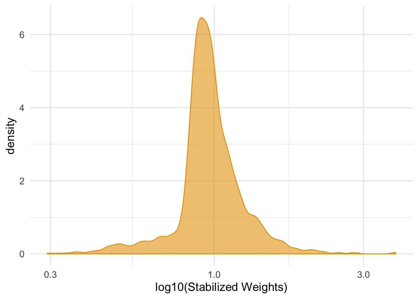

lm_robust(wt82_71 ~ qsmk*sex, data = nhefs_complete, weights = swts) %>% 
  tidy()

##          term     estimate std.error   statistic      p.value   conf.low
## 1 (Intercept)  1.784446876 0.3101597  5.75331559 1.051124e-08  1.1760735
## 2        qsmk  3.521977634 0.6585705  5.34791301 1.021696e-07  2.2302023
## 3        sex1 -0.008724784 0.4492401 -0.01942121 9.845076e-01 -0.8899019
## 4   qsmk:sex1 -0.159478525 1.0498718 -0.15190286 8.792832e-01 -2.2187851
##   conf.high   df outcome
## 1 2.3928202 1562 wt82_71
## 2 4.8137530 1562 wt82_71
## 3 0.8724524 1562 wt82_71
## 4 1.8998280 1562 wt82_71

2.7 Program 12.7

# using complete data set
nhefs_censored <- nhefs %>% 
  drop_na(qsmk, sex, race, age, school, smokeintensity, smokeyrs, exercise, 
         active, wt71)

numerator_sws_model <- glm(qsmk ~ 1, data = nhefs_censored, family = binomial())

numerators_sws <- numerator_sws_model %>% 
  augment(type.predict = "response", data = nhefs_censored) %>% 
  mutate(numerator_sw = ifelse(qsmk == 0, 1 - .fitted, .fitted)) %>% 
  select(id, numerator_sw)

denominator_sws_model <- glm(
  qsmk ~ sex + race + age + I(age^2) + education + 
  smokeintensity + I(smokeintensity^2) + 
  smokeyrs + I(smokeyrs^2) + exercise + active + 
  wt71 + I(wt71^2), 
  data = nhefs_censored, family = binomial()
)

denominators_sws <- denominator_sws_model %>% 
  augment(type.predict = "response", data = nhefs_censored) %>% 
  mutate(denominator_sw = ifelse(qsmk == 0, 1 - .fitted, .fitted)) %>% 
  select(id, denominator_sw)

numerator_cens_model <- glm(censored ~ qsmk, data = nhefs_censored, family = binomial())

numerators_cens <- numerator_cens_model %>% 
  augment(type.predict = "response", data = nhefs_censored) %>% 
  mutate(numerator_cens = ifelse(censored == 0, 1 - .fitted, 1)) %>% 
  select(id, numerator_cens)

denominator_cens_model <- glm(
  censored ~ qsmk + sex + race + age + I(age^2) + education + 
  smokeintensity + I(smokeintensity^2) + 
  smokeyrs + I(smokeyrs^2) + exercise + active + 
  wt71 + I(wt71^2), 
  data = nhefs_censored, family = binomial()
)

denominators_cens <- denominator_cens_model %>% 
  augment(type.predict = "response", data = nhefs_censored) %>% 
  mutate(denominator_cens = ifelse(censored == 0, 1 - .fitted, 1)) %>% 
  select(id, denominator_cens)

nhefs_censored_wts <- nhefs_censored %>% 
  left_join(numerators_sws, by = "id") %>% 
  left_join(denominators_sws, by = "id") %>% 
  left_join(numerators_cens, by = "id") %>% 
  left_join(denominators_cens, by = "id") %>% 
  mutate(
    swts = numerator_sw / denominator_sw, 
    cens_wts = numerator_cens / denominator_cens,
    wts = swts * cens_wts
  )

nhefs_censored_wts %>% 
  summarize(mean_wt = mean(cens_wts), sd_wts = sd(cens_wts))

## # A tibble: 1 x 2
##   mean_wt sd_wts
##     <dbl>  <dbl>
## 1   0.999 0.0519

ggplot(nhefs_censored_wts, aes(cens_wts)) +
  geom_density(col = "#E69F00", fill = "#E69F0095") + 
  scale_x_log10() + 
  theme_minimal(base_size = 14) + 
  xlab("log10(Stabilized Weights)")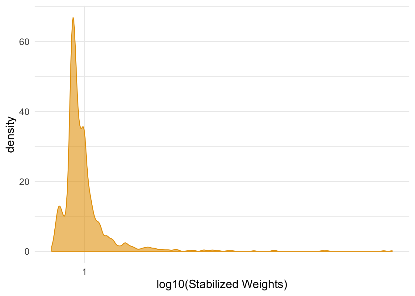

lm_robust(wt82_71 ~ qsmk, data = nhefs_censored_wts, weights = wts) %>% 
  tidy()

##          term estimate std.error statistic      p.value conf.low conf.high
## 1 (Intercept) 1.661990 0.2328693  7.137009 1.454358e-12 1.205221  2.118759
## 2        qsmk 3.496493 0.5265564  6.640301 4.305944e-11 2.463662  4.529324
##     df outcome
## 1 1564 wt82_71
## 2 1564 wt82_71